| team | opponent | is_home | goals |
|---|---|---|---|
| Arsenal | Chelsea | 1 | 1 |
| Chelsea | Arsenal | 0 | 0 |
Arsenal 1–0 Chelsea, 2025-03-16
In a football match, goals are simply events that occur at some random, steady average rate. That is exactly what the Poisson distribution specialises in predicting. So for any given match, this model reduces to a simple question: what is each team’s average goal rate?
The dataset is nine seasons of Premier League results plus Bet365 closing odds. Each match in the dataset is immediately split into two rows, with both the home and away side appearing as “team” and “opponent”. An example:
| team | opponent | is_home | goals |
|---|---|---|---|
| Arsenal | Chelsea | 1 | 1 |
| Chelsea | Arsenal | 0 | 0 |
Arsenal 1–0 Chelsea, 2025-03-16
Because each team now appears as both the scorer and the conceder, a single regression can learn attack and defence for all 34 teams simultaneously.
A team’s goal rate is built from four distinct numbers: the baseline (0.312) — what an average team scores against an average team (about 1.3 goals); home advantage (0.192) — playing at home increases your goal rate by roughly 21%; attack — a number per team which, if positive, means they score more than average; defence — a number per team that, if positive, means they concede more than average.
So, in order to predict one fixture, we must calculate λ_home = exp(baseline + home_advantage + attack[home] + defence[away]) and λ_away = exp(baseline + attack[away] + defence[home]). The only difference between the formulas is that the away side does not get the home-advantage coefficient.
In order to convert these numbers into probabilities, we assume that each side’s goal count is Poisson-distributed with its own λ, and that the two sides are independent of each other. Under independence, the probability of any scoreline is just the two probabilities multiplied: P(2–1) = P(home scores 2) × P(away scores 1). Do that for every combination and you get a grid:
| 0 | 1 | 2 | 3 | 4 | 5 | |
|---|---|---|---|---|---|---|
| 0 | 7.4 | 9.8 | 6.5 | 2.9 | 0.9 | 0.3 |
| 1 | 9.4 | 12.5 | 8.3 | 3.7 | 1.2 | 0.3 |
| 2 | 6.1 | 8.0 | 5.3 | 2.4 | 0.8 | 0.2 |
| 3 | 2.6 | 3.4 | 2.3 | 1.0 | 0.3 | 0.1 |
| 4 | 0.8 | 1.1 | 0.7 | 0.3 | 0.1 | 0.0 |
| 5 | 0.2 | 0.3 | 0.2 | 0.1 | 0.0 | 0.0 |
Sum the coloured regions and we get three market prices:
P(Wolves win) = 35.8%, P(draw) = 26.3%, P(Brentford win) = 37.8%
Now, there is a flaw in this method: the independence assumption is an issue. In a real match, the actions (goals) of one team certainly affect the other — if a team goes 2–0 up away from home they will likely choose to sit back and not risk any more, or, inversely, a team losing 2–0 at home would play far more open and aggressive, chasing a goal. To fix this you would implement Dixon-Coles, which is a small correction factor for low-scoring games. To be clear, Dixon-Coles is not implemented in this model yet.
Pick any two teams from the training set — expected goals, the scoreline grid, and the derived markets below recompute live from the model’s fitted coefficients, in a few KB of plain JavaScript (no page reload, no framework runtime).
| Market | Probability |
|---|
Loading model coefficients…
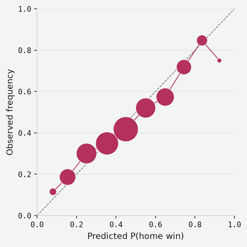
So… does it work? To see how we did, we compare ourselves to the Bet365 closing price for all of these matches — with one wrinkle: if you total the three markets Bet365 offers per game, they sum to roughly 105%, which is the bookmaker’s edge. We have to devig these prices to make the comparison with my model fair. The comparison uses two “scores”: log loss (which asks “how surprised were you by what actually happened?” — it punishes being confidently wrong very harshly) and Brier score (a squared error between your probability and the outcome).
“Backtested against the closing line” means specifically this: the model is refit once per season, never mid-season, on every season strictly before the one it’s about to predict — 2016/17 through 2018/19 is training-only and never scored itself, then 2019/20 gets predicted using only 2016/17–2018/19, 2020/21 using only the seasons before it, and so on through 2024/25. That’s an expanding window, not a rolling one — nothing already in training ever ages out or gets dropped as the window moves forward. Every match inside a given season is scored off that same season-start fit; the coefficients aren’t touched again until the next season’s matches start. 298 matches get skipped rather than scored, because they involve a team with no result in the training data yet (mostly clubs freshly promoted into the league) — the model has no attack/defence rating to predict from for a team it’s never seen play.
| Metric | Model | Market (Bet365, devigged) |
|---|---|---|
| n | 1982 | |
| Log loss | 1.004 | 0.961 |
| Brier score | 0.598 | 0.569 |
The market beat my model on both. This is expected — there are numerous limitations to this model beyond just missing Dixon-Coles. It includes no time-decay weighting and no injury or lineup information, yet it still landed within a few percent of a market that has millions of people betting on it every week.